Note
This page was generated from a Jupyter notebook. To run and interact with it,
you can download it here.
Regression modelling
This notebook works through an example showing how homonim can improve regression performance. It uses aerial imagery and ground truth data from a study that investigated aboveground carbon (AGC) mapping in the thicket biome, South Africa.
Aerial imagery consists of 4 50cm resolution, 4 band images, captured on 8-9 May 2015, covering a small site in the Baviaanskloof. The images are orthorecified but otherwise unadjusted i.e. without colour balancing, gamma correction etc. Imagery was captured and supplied by NGI. Ground truth consists of AGC estimates and polygons for 85 plots. This dataset is licensed under the terms of the CC BY-NC-SA 4.0.
Reference imagery is acquired using geedim.
APIs of homonim and other packages are used. CLI commands equivalent to the API code snippets are given in the comments where possible.
Setup
geedim, geopandas, gdal and matplotlib are required to run the notebook. You can uncomment the cell below to install them, if they aren’t installed already.
[1]:
# import sys
# if 'conda' in sys.prefix:
#     # install into the conda environment the notebook is being run from
#     !conda install --yes --prefix {sys.prefix} -c conda-forge geedim geopandas gdal matplotlib
# else:
#     # install into the python environment the notebook is being run from
#     !{sys.executable} -m pip install geedim geopandas gdal matplotlib
[2]:
# imports used by more than one cell
import logging
import warnings
from pathlib import Path
from matplotlib import pyplot
import numpy as np
import rasterio as rio
from tqdm.auto import tqdm

import geedim as gd
from homonim.errors import HomonimWarning

# keep notebook free of homonim logs / warnings
logging.basicConfig(level=logging.ERROR)
warnings.simplefilter('ignore', category=HomonimWarning)
Download aerial images
In this step, we download & extract the source aerial images into an images sub-folder. The image download is large (~ 2 GB), so you can do this step manually if you prefer.
[3]:
from zipfile import ZipFile
from urllib import request

# set up url, images directory, and download file name
src_url = 'https://zenodo.org/record/7130228/files/Ngi_May2015_Source.zip'
images_path = Path('images')
images_path.mkdir(exist_ok=True)
zip_path = images_path.joinpath('temp.zip')

# download zip file if it doesn't exist
if not zip_path.exists():
    response = request.urlopen(src_url)
    with tqdm(
        total=response.length, desc='Download', unit='B', unit_scale=True,
        dynamic_ncols=True
    ) as pbar, open(zip_path, 'wb')  as fout:
        for chunk in response:
            fout.write(chunk)
            pbar.update(len(chunk))

# extract zip file
with ZipFile(zip_path) as zip_file:
     for file in tqdm(
        zip_file.namelist(), desc='Extract', dynamic_ncols=True
    ):
        zip_file.extract(member=file, path=images_path)
Search for reference image
Next, we search for a suitable Sentinel-2 reference image using geedim. Sentinel-2 is chosen for its relatively high resolution (10m), and bands that are spectrally similar to the aerials.
Normally it is best to search for a reference that is concurrent with the source imagery, but in this example, the Sentinel-2 archive begins after the source capture date (8-9 May 2015). As a compromise, we search for the soonest possible reference after the source capture date.
[4]:
gd.Initialize()  # initialise the earth engine API
src_mosaic_path = Path('images/Ngi_May2015_OrthoNgiDem_Source_Mosaic.vrt')

# create a search region that covers the source image mosaic
region = gd.utils.get_bounds(src_mosaic_path)

# create and search the earth engine Sentinel-2 collection
s2_coll = gd.MaskedCollection.from_name('COPERNICUS/S2')
s2_coll = s2_coll.search('2015-05-08', '2015-10-30', region, cloudless_portion=0)
print('Image property descriptions:\n\n' + s2_coll.schema_table)
print('\nSearch Results:\n\n' + s2_coll.properties_table)

# equivalent geedim command line:
#!geedim search -c s2-toa -s 2015-05-08 -e 2015-10-30 -r {src_mosaic_path} -cp 50
Image property descriptions:

ABBREV     NAME                             DESCRIPTION
---------  -------------------------------  ----------------------------------------------
ID         system:id                        Earth Engine image id
DATE       system:time_start                Image capture date/time (UTC)
FILL       FILL_PORTION                     Portion of region pixels that are valid (%)
CLOUDLESS  CLOUDLESS_PORTION                Portion of filled pixels that are cloud/shadow
                                            free (%)
RADQ       RADIOMETRIC_QUALITY              Radiometric quality check
GEOMQ      GEOMETRIC_QUALITY                Geometric quality check
SAA        MEAN_SOLAR_AZIMUTH_ANGLE         Solar azimuth angle (deg)
SZA        MEAN_SOLAR_ZENITH_ANGLE          Solar zenith angle (deg)
VAA        MEAN_INCIDENCE_AZIMUTH_ANGLE_B1  View (B1) azimuth angle (deg)
VZA        MEAN_INCIDENCE_ZENITH_ANGLE_B1   View (B1) zenith angle (deg)

Search Results:

ID                                                   DATE             FILL CLOUDLESS RADQ   GEOMQ    SAA   SZA    VAA  VZA
---------------------------------------------------- ---------------- ---- --------- ------ ------ ----- ----- ------ ----
COPERNICUS/S2/20150913T080256_20150913T082256_T34HGH 2015-09-13 08:22  100      5.55 PASSED PASSED 40.34 45.99  99.34 4.69
COPERNICUS/S2/20150913T080256_20150913T082256_T35HKC 2015-09-13 08:22  100      5.36 PASSED PASSED 39.65 45.68 179.46 3.06
COPERNICUS/S2/20150913T080256_20161230T054320_T34HGH 2015-09-13 08:22  100      5.58 PASSED PASSED 40.34 45.99  99.34 4.69
COPERNICUS/S2/20150913T080256_20161230T054320_T35HKC 2015-09-13 08:22  100      5.32 PASSED PASSED 39.65 45.68 179.46 3.06
COPERNICUS/S2/20151003T075826_20151003T082014_T34HGH 2015-10-03 08:20  100      5.97 PASSED PASSED 44.69 38.60  99.44 4.68
COPERNICUS/S2/20151003T075826_20151003T082014_T35HKC 2015-10-03 08:20  100      5.90 PASSED PASSED 43.92 38.26 180.55 3.06
COPERNICUS/S2/20151003T075826_20161206T031927_T34HGH 2015-10-03 08:20  100      5.97 PASSED PASSED 44.69 38.60  99.44 4.68
COPERNICUS/S2/20151003T075826_20161206T031927_T35HKC 2015-10-03 08:20  100      5.90 PASSED PASSED 43.92 38.26 180.55 3.06
COPERNICUS/S2/20151023T081112_20151023T081949_T34HGH 2015-10-23 08:19  100    100.00 PASSED PASSED 51.10 32.03 100.32 4.60
COPERNICUS/S2/20151023T081112_20151023T081949_T35HKC 2015-10-23 08:19  100    100.00 PASSED PASSED 50.27 31.65 183.14 3.07
COPERNICUS/S2/20151023T081112_20161216T015401_T34HGH 2015-10-23 08:19  100    100.00 PASSED PASSED 51.10 32.03 100.32 4.60
COPERNICUS/S2/20151023T081112_20161216T015401_T35HKC 2015-10-23 08:19  100    100.00 PASSED PASSED 50.27 31.65 183.14 3.07
Download reference image
Now, using geedim again, we download the first 100% cloudless Sentinel-2 image - COPERNICUS/S2/20151023T081112_20151023T081949_T34HGH.
[5]:
ref_path = Path('images/s2_reference.tif')
gd_image = gd.MaskedImage.from_id(
    'COPERNICUS/S2/20151023T081112_20151023T081949_T34HGH', mask=True
)
gd_image.download(ref_path, region=region, overwrite=True)

# equivalent geedim command line:
# !geedim download -i COPERNICUS/S2/20151023T081112_20151023T081949_T34HGH --mask -r {src_mosiac_path}
Surface reflectance correction
Here, we correct the aerial images by fusion with the Sentinel-2 reference. We use homonim’s RasterFuse class, the gain-blk-offset model, and a kernel shape of 15 x 15 pixels. The model and kernel shape values were chosen through trial and error as the ones producing the best regression performance.
The source images are not RGB, and do not have center_wavelength data, meaning RasterFuse cannot auto-match source and reference bands. Sentinel-2 bands corresponding to the red, green, blue and NIR of the source images are specified with the ref_bands parameter in the call to RasterFuse().
[6]:
from homonim import RasterFuse, Model

# paths to source aerial images
src_paths = [
    Path(f'images/3323d_2015_1001_02_00{i}_RGBN_CMP.tif')
    for i in [76, 78, 80, 81]
]
# paths to corrected images to create
corr_paths = [
    src_path.parent.joinpath(f'{src_path.stem}_FUSE.tif')
    for src_path in src_paths
]
[7]:
# sentinel-2 bands that correpond to the red, green, blue and near-infrared bands of
# the aerial images
ref_bands = [4, 3, 2, 8]

# specify a uint16 dtype and nodata value of 0 for the corrected files
out_profile = RasterFuse.create_out_profile(dtype='uint16', nodata=0)

# iterate over source and corrected paths
for src_path, corr_path in zip(src_paths, corr_paths):
    with RasterFuse(
        src_path, ref_path, ref_bands=ref_bands
    ) as raster_fuse:
        raster_fuse.process(
            corr_path, Model.gain_blk_offset, (15, 15), overwrite=True,
            out_profile=out_profile,
        )

        # equivalent homonim command line:
        # !homonim fuse -m gain-blk-offset -k 15 15 -rb 4 -rb 3 -rb 2 -rb 8 -od images {src_path} {ref_path}
Next, we create a VRT mosaic of the corrected images to use in the visualisation and evaluation sections.
[8]:
# strictly, one should avoid using GDAL and rasterio together, but it doesn't
# create conflicts here
from osgeo import gdal
gdal.UseExceptions()

corr_mosaic_path = Path('images/Ngi_May2015_OrthoNgiDem_Corrected_Mosaic.vrt')
ds = gdal.BuildVRT(
    str(corr_mosaic_path.absolute()), [str(cp) for cp in corr_paths]
)
_ = ds.FlushCache()
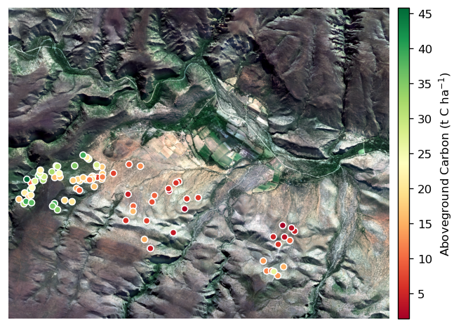
Visualisation
In this section we produce a map of the AGC ground truth values and locations on the corrected image mosaic. We start by loading the AGC ground truth into a geopandas GeoDataFrame.
[9]:
import geopandas as gpd

plot_agc_gdf = gpd.GeoDataFrame.from_file(
    'https://raw.githubusercontent.com/leftfield-geospatial/map-thicket-agc/main/'
    'data/outputs/geospatial/gef_plot_polygons_with_agc_v2.gpkg'
)
Then we create and format the map.
[10]:
from rasterio.plot import show
from mpl_toolkits.axes_grid1 import make_axes_locatable

indexes = [1, 2, 3]  # red, green, blue band indices
ds_fact = 4  # factor by which to downsample bands

fig, ax = pyplot.subplots(1, 1, tight_layout=True, figsize=(6, 4), dpi=120)
divider = make_axes_locatable(ax)
cax = divider.append_axes('right', size='3%', pad=0.1)

# read, normalise and display corrected mosaic
with rio.open(corr_mosaic_path, 'r') as corr_ds:
    # downsampled band shape & transform
    ds_shape = tuple(np.round(np.array(corr_ds.shape) / ds_fact).astype('int'))
    transform = corr_ds.transform * rio.Affine.scale(ds_fact)

    # read image and downsample
    array = corr_ds.read(
        indexes=indexes, out_dtype='float32', out_shape=ds_shape
    )

    # change nodata value to nan
    mask = np.any(array == corr_ds.nodata, axis=(0))
    array[:, mask] = np.nan

    # 'normalise' image 2%-98% -> 0-1
    for bi in range(len(indexes)):
        array[bi] -= np.nanpercentile(array[bi], 2)
        array[bi] /= np.nanpercentile(array[bi], 98)
        array[bi] = np.clip(array[bi], 0, 1)

    ax = show(array, transform=transform, interpolation='bilinear', ax=ax)

# plot colour coded points for each AGC ground truth plot
_plot_agc_gdf = plot_agc_gdf.to_crs(corr_ds.crs)
_plot_agc_gdf.geometry = _plot_agc_gdf.geometry.centroid
_plot_agc_gdf.AgcHa /= 1000
ax = _plot_agc_gdf.plot(
    'AgcHa', kind='geo', legend=True, ax=ax, cmap='RdYlGn', cax=cax, edgecolor='white',
    legend_kwds=dict(label='Aboveground Carbon (t C ha$^{-1}$)', orientation='vertical'),
    linewidth=1, markersize=30,
)

# zoom in
_ = ax.axis((86494.06047619047, 94313.07562770562, -3717680.7510822513, -3711286.8766233767))
_ = ax.axis('off')
# fig.savefig('../case_studies/regression_modelling-agc_map.jpg', dpi=120)
Evaluation
The evaluation compares the correlation of source and corrected NDVI with AGC ground truth. From this basic comparison, we have an indication of the improvement in the relevance, or explanatory power of the image due to surface reflectance correction. While NDVI is well correlated with AGC in this problem, it used just for demonstration purposes. There may be other spectral indices and image features that better explain AGC.
To start, we find the mean NDVI values for each ground truth plot, for both source and corrected images.
[11]:
from rasterio import features, windows
from homonim import utils

src_mosaic_path = Path('images/Ngi_May2015_OrthoNgiDem_Source_Mosaic.vrt')
ndvis = []

# iterate over source and corrected mosaics
for im_path in [src_mosaic_path, corr_mosaic_path]:
    ndvi = []
    with rio.open(im_path, 'r') as ds:
        # loop over ground truth plots
        for id, plot in tqdm(
            plot_agc_gdf.to_crs(ds.crs).iterrows(), total=plot_agc_gdf.shape[0],
            desc=im_path.name, dynamic_ncols=True,
        ):
            # find a rasterio window that contains the plot polygon
            bounds = features.bounds(plot.geometry)
            win = windows.from_bounds(*bounds, transform=ds.transform)
            win = utils.expand_window_to_grid(win)

            # read the image array corresponding to the plot window
            array = ds.read(out_dtype='float64', window=win)

            # find a mask for pixels contained inside the plot polygon
            win_transform = ds.window_transform(win)
            mask = ~features.geometry_mask(
                plot.geometry.geoms, (win.height, win.width), transform=win_transform
            )

            # find mean NDVI for the plot
            r = array[0, mask]
            nir = array[3, mask]
            ndvi.append(np.mean((nir - r) / (nir + r)))

    ndvis.append(ndvi)

ndvi_dict = dict(zip(['Source', 'Corrected'], ndvis))
Then we create scatter plots of source / corrected NDVI vs. AGC, and display the corresponding \(r^2\) correlation coefficients.
[12]:
fig, axes = pyplot.subplots(1, 2, tight_layout=True, figsize=(8, 4), dpi=100)
agc = plot_agc_gdf.AgcHa / 1000

# iterate over source & corrected axes, labels & ndvi values
for ax, (label, ndvi) in zip(axes, ndvi_dict.items()):
    # plot NDVI vs AGC scattter
    ax.plot(ndvi, agc, '.')

    # find and plot regression line
    coeff, _, _, _ = np.linalg.lstsq(
        np.array([ndvi, np.ones(len(ndvi))]).T, agc, rcond=None
    )
    xlim = [np.min(ndvi), np.max(ndvi)]
    ylim = [np.min(agc), np.max(agc)]
    yr = np.array(xlim) * coeff[0] + coeff[1]
    ax.plot(xlim, yr, 'k--', lw=2, zorder=-1)

    # find R2 correlation coefficient and add to plot
    r2 = np.corrcoef(agc, ndvi)[0, 1] **2
    ax.text(
        .1, 0.9, f'$r^{2}={r2:.2f}$', transform=ax.transAxes,
        fontweight='bold'
    )

    ax.set_xlabel('NDVI')
    ax.set_ylabel('AGC (t C ha$^{-1}$)')
    ax.set_xlim(xlim)
    ax.set_ylim(ylim)
    ax.set_title(label, fontweight='bold')

# fig.savefig(
#     'regression_modelling-eval.png', facecolor='white',
#     transparent=False, dpi=92,
# )
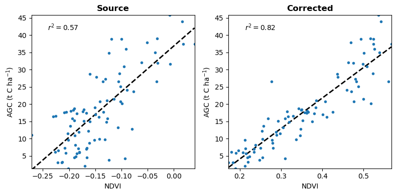
Surface reflectance correction improves the relevance of NDVI for prediciting AGC.
Note
Details on the data and original study can be found in the related github repository and paper.